Why physics-based?¶

The name “Thermodynamic Models for Heat Pumps” describes what tmhp is — a library of thermodynamic cycle models. How those models are written is the part this page is about: every cycle is solved from first principles, not fitted against catalogue data.

Most building-energy simulators take the opposite route. They model a heat pump as an empirical curve fit — typically a polynomial in (outdoor temperature, leaving-water temperature) calibrated against the manufacturer’s test points. That approach is cheap and accurate inside the calibration envelope, but it carries three structural limitations that this library was built to remove.

The three structural limits of curve fits¶

	Curve-fit models	`tmhp`
Operating range	Tied to the manufacturer’s test points; extrapolation is unreliable.	Predictive across the full refrigerant envelope — limited by the EOS, not by training data.
Refrigerant	Baked into the fitted coefficients. Changing R410A → R290 requires a new dataset.	The refrigerant is a constructor argument (`ref="R290"`). Anything CoolProp supports works.
State visibility	Cycle state is hidden behind the fit. You see COP; you don’t see why.	Every cycle node (compressor in/out, expander in/out, evaporator / condenser saturation) is in the result frame at every step.

Same envelope, two different sources¶

The figure below sweeps the heat-source inlet temperature for an ASHP (source = outdoor air) and a GSHP (source = ground-loop fluid) at the same condenser duty and tank set-point. Both curves come straight out of analyze_steady with no fitted coefficients — the COP shape, including the steep ASHP drop below freezing, falls out of the EOS through the compressor and heat-exchanger models.

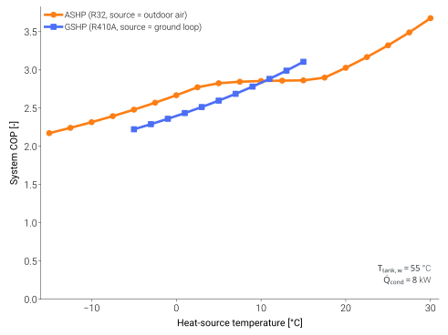
System COP for an ASHP and a GSHP as a function of the heat-source inlet temperature, at fixed tank set-point and condenser duty. — System COP versus heat-source inlet temperature. The GSHP curve spans the narrow stable range of a ground loop; the ASHP curve extends across the wide but COP-eroding range of outdoor air. Generated by `scripts/visualization/cop_vs_source_temp.py`.¶

What gets solved at every time step¶

Each call to analyze_steady (and each step of analyze_dynamic) solves a closed refrigerant cycle coupled to the surrounding system. The condenser duty is the target; the evaporating temperature is found by internally minimising compressor power, so the cycle closes on a physical optimum rather than on fitted coefficients.

Sub-model	Method
Refrigerant state points	CoolProp (REFPROP-grade EOS).
Compressor work	Isentropic + volumetric + mechanical efficiency.
Condenser / evaporator	ε-NTU heat exchanger model.
Outdoor unit fan	ASHRAE 90.1-style VSD power curve, air-side ε-NTU.
Borehole (GSHP)	g-function via pygfunction.
PV / solar thermal	pvlib-driven irradiance and power.
Cycle closure	Internal minimisation → optimal evaporating temperature.

The same core cycle is reused across every system model — what changes is the source side (air / ground / water) and the sink side (DHW tank, building load, or hybrid PV / STC / ESS).

The compute trade-off¶

Solving an EOS state at every cycle node is more expensive than evaluating a polynomial. In practice it lands around a few hundred steps per second on a single core for a vanilla ASHPB — fast enough that a year-long minute-resolution run takes hours, not minutes.

If that is still too slow for your use case, a fitted surrogate is the right escape hatch. tmhp tracks commercial catalogue data well enough (see Validation) that you can train the surrogate against this library itself, without collecting fresh bench data.