Realistic dynamic simulation¶

Your first dynamic simulation runs analyze_dynamic with flat schedules — a clean sanity check, but real runs almost never look like that.

This tutorial assembles a more representative 24-hour scenario:

a domestic-hot-water draw profile with morning and evening peaks;
a sinusoidal outdoor-temperature schedule (overnight low, mid-afternoon high);
and CSV output for downstream analysis.

What a real day looks like¶

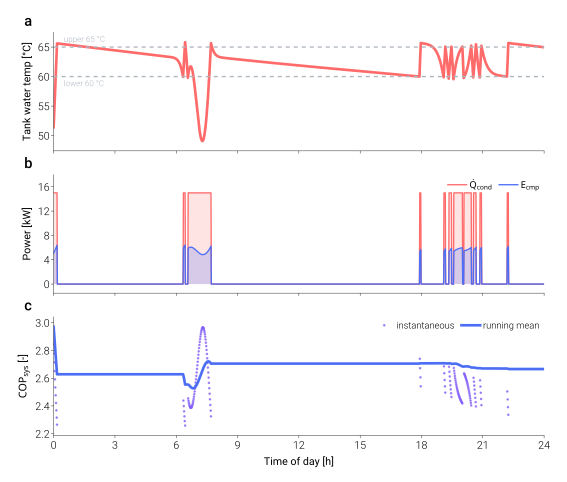
24-hour dynamic simulation of the ASHPB. Three stacked panels — tank temperature with its upper/lower bounds, condenser heat rate and compressor electrical power, and instantaneous + running-mean system COP. — 24-hour ASHPB run with two DHW draws (07:00 and 20:00) and a sinusoidal outdoor temperature. Generated by `scripts/visualization/dynamic_24h_timeseries.py`.¶

The schedule arrays¶

import numpy as np

simulation_period_sec = 24 * 3600
dt_s                  = 60
n_steps               = simulation_period_sec // dt_s
minute_of_day         = np.arange(n_steps)
hour_of_day           = minute_of_day / 60.0

# Outdoor temperature: cosine, low at ~05:00, high at ~17:00 (12 h shift)
T0_mean      = 5.0     # °C — daily mean
T0_amplitude = 8.0     # ±°C
T0_schedule  = T0_mean - T0_amplitude * np.cos(
    2 * np.pi * (hour_of_day - 5.0) / 24.0,
)

# DHW draw: two gaussian peaks (~07:00 and ~19:00).
# 100 L over the day, spread across the two peaks.
def gaussian_peak(center_h, sigma_h, total_volume_m3):
    weight = np.exp(-0.5 * ((hour_of_day - center_h) / sigma_h) ** 2)
    weight /= weight.sum()
    return weight * (total_volume_m3 / dt_s)   # m³/s per step

dhw_morning = gaussian_peak(center_h=7.0,  sigma_h=0.6, total_volume_m3=0.040)
dhw_evening = gaussian_peak(center_h=19.0, sigma_h=0.8, total_volume_m3=0.060)
dhw_usage_schedule = dhw_morning + dhw_evening

Running and saving¶

from tmhp import AirSourceHeatPumpBoiler

ashpb = AirSourceHeatPumpBoiler(ref="R32")

df = ashpb.analyze_dynamic(
    simulation_period_sec = simulation_period_sec,
    dt_s                  = dt_s,
    T_tank_w_init_C       = 55.0,
    dhw_usage_schedule    = dhw_usage_schedule,
    T0_schedule           = T0_schedule,
    result_save_csv_path  = "run_realistic.csv",
)

result_save_csv_path writes the per-step DataFrame to disk in the same shape as the returned object — convenient for piping into pandas / Excel without re-running the simulation.

Inspecting the run¶

# Energy balance over the day
E_cmp_kWh   = df["E_cmp [W]"].sum() * dt_s / 3.6e6
Q_cond_kWh  = df["Q_ref_cond [W]"].sum() * dt_s / 3.6e6
cop_sys_avg = df["cop_sys [-]"].mean()

print(f"Total compressor energy  : {E_cmp_kWh:5.2f} kWh")
print(f"Total condenser duty     : {Q_cond_kWh:5.2f} kWh")
print(f"Daily-average COP_sys    : {cop_sys_avg:5.2f}")

# When did the heat pump struggle?
from collections import Counter
print(Counter(df["failure_reason"]))

The Counter gives a quick view of how many steps hit each diagnostic. For a sensible system at moderate ambient, almost every step should be none — see failure_reason semantics for what the other values mean.

Where to go next¶

Replace the synthetic outdoor schedule with real weather data resampled to your dt_s.
Drive a multi-day or annual run by concatenating schedules and passing the longer simulation_period_sec.
Plug in subsystems (STC, PV/ESS) — see Air-source heat pump boiler (ASHPB).