Visualize thermodynamic cycle

Because tmhp solves the cycle from first principles, every analyze_steady call returns the full thermodynamic state at each cycle node (compressor in / out, expander in / out, evaporator / condenser saturation). Plotting those points on a pressure–enthalpy (P–h) chart — and, side by side, on a temperature–enthalpy (T–h) chart — is the fastest way to sanity-check a solved cycle.

This tutorial draws both panels with no extra dependencies — just CoolProp and Matplotlib, both already pulled in by uv sync.

The output

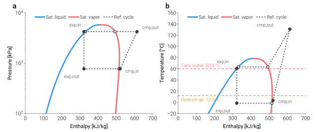
R32 cycle at a realistic DHW operating point — \(T_{\mathrm{tank}}=60\,^{\circ}\mathrm{C}\), \(T_{0}=12\,^{\circ}\mathrm{C}\), \(\dot{Q}_{\mathrm{cond}}=8\,\mathrm{kW}\). Filled circles are the four cycle states (cmp,in / cmp,out / exp,in / exp,out); open circles are the saturation-envelope crossings. Panel (b) overlays the tank-water and outdoor-air temperatures as the heat-sink and heat-source references.

The T-s companion view

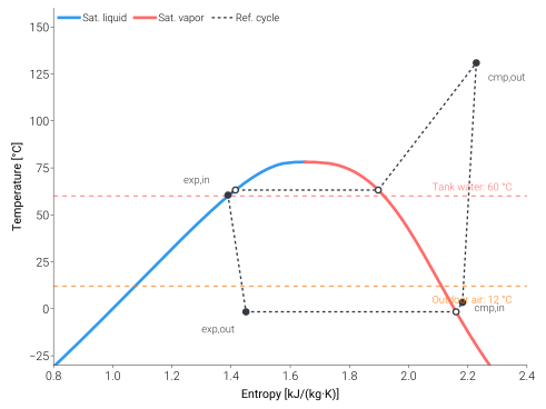
Same cycle, plotted on a T-s plane. Compression (1→2) is a near-vertical climb (the cycle is close to isentropic), while isenthalpic expansion (3→4) generates entropy and sits visibly to the right of point 3 on the saturation dome.

How to read it

• Saturation envelope — blue is saturated liquid, red is saturated vapour. The dome interior is two-phase; outside is single-phase liquid (left) or vapour (right).

• Cycle traversal — follow the four labelled states in order:

  • exp,out → cmp,in — evaporation at the source side. Horizontal segment on the P–h panel at the evaporating pressure; the T–h panel shows it tracking just above the outdoor-air reference line.

  • cmp,in → cmp,out — compression. Pressure climbs sharply; enthalpy increases by the specific work of the compressor.

  • cmp,out → exp,in — de-superheat + condensation at the condenser pressure. Enthalpy drops as the refrigerant gives up its latent heat to the water side; the T–h panel shows it settling just above the tank-water reference line.

  • exp,in → exp,out — isenthalpic expansion. Vertical segment on the P–h panel (h preserved, pressure drops); the T–h panel shows the corresponding temperature drop down to the evaporating temperature.

The script

The complete script lives at scripts/visualization/mollier_cycle_R32.py. The core is a saturation-envelope sweep via CoolProp for each panel plus a dashed connector through the seven cycle points returned by analyze_steady:

import CoolProp.CoolProp as CP
import matplotlib.pyplot as plt
import numpy as np

from tmhp import AirSourceHeatPumpBoiler

REF = "R32"
ashpb = AirSourceHeatPumpBoiler(ref=REF)
r = ashpb.analyze_steady(T_tank_w=60.0, T0=12.0, Q_ref_cond=8_000.0)

# Saturation envelope for the P-h panel (kJ/kg, kPa).
T_crit = CP.PropsSI("Tcrit", REF)
T_grid = np.linspace(220.0, T_crit - 0.5, 200)
h_liq = np.array([CP.PropsSI("H", "T", T, "Q", 0, REF) for T in T_grid]) / 1_000
h_vap = np.array([CP.PropsSI("H", "T", T, "Q", 1, REF) for T in T_grid]) / 1_000
p_sat = np.array([CP.PropsSI("P", "T", T, "Q", 0, REF) for T in T_grid]) / 1_000

def hp(h_key, p_key):
    return r[h_key] / 1_000, r[p_key] / 1_000

pts = {
    "1*": hp("h_ref_evap_sat [J/kg]",   "P_ref_evap_sat [Pa]"),
    "1":  hp("h_ref_cmp_in [J/kg]",     "P_ref_cmp_in [Pa]"),
    "2":  hp("h_ref_cmp_out [J/kg]",    "P_ref_cmp_out [Pa]"),
    "2*": hp("h_ref_cond_sat_v [J/kg]", "P_ref_cond_sat_v [Pa]"),
    "3*": hp("h_ref_cond_sat_l [J/kg]", "P_ref_cond_sat_l [Pa]"),
    "3":  hp("h_ref_exp_in [J/kg]",     "P_ref_exp_in [Pa]"),
    "4":  hp("h_ref_exp_out [J/kg]",    "P_ref_exp_out [Pa]"),
}

fig, ax = plt.subplots(figsize=(7.2, 5.0))
ax.plot(h_liq, p_sat, label="Sat. liquid")
ax.plot(h_vap, p_sat, label="Sat. vapor")

path = ["1*", "1", "2", "2*", "3*", "3", "4", "1*"]
xs = [pts[p][0] for p in path]
ys = [pts[p][1] for p in path]
ax.plot(xs, ys, marker="o", linestyle=":", label="Ref. cycle")

ax.set_yscale("log")
ax.set_xlabel("Enthalpy [kJ/kg]")
ax.set_ylabel("Pressure [kPa]")
ax.legend()

The full script in the repo extends this minimal core with the T–h panel, the operating-condition reference lines, and the open / filled marker convention used in the figure above.

To regenerate the figure shipped with the docs:

uv sync --locked
uv run python scripts/visualization/mollier_cycle_R32.py

The script pins mpl.rcParams["svg.hashsalt"] so the resulting SVG is byte-identical across runs — the same convention used by scripts/validation/samsung_ehs_parity.py.

Going further

• Other refrigerants — change REF (and re-run analyze_steady with the same operating point) to compare cycle shapes across R290, R410A, R134a, etc.

• Other diagrams — the library also ships a mollier_diagram module with T–h, P–h, and T–s plotters in Visualization. These are styled with dartwork-mpl, a thin matplotlib utility layer that is pulled in automatically by uv sync.

• Multi-point overlays — pass several analyze_steady results to the same figure to compare cycles at different outdoor temperatures or different LWT set-points.

Last updated May 19, 2026