Your first dynamic simulation

For ASHPB, analyze_dynamic solves the same refrigerant cycle as analyze_steady at every time step, coupled to a tank-energy balance and any active subsystems. This page walks through the simplest possible call — 24 hours of operation against a constant outdoor temperature and zero DHW draw — so you can see the shape of the per-step result before adding realistic schedules in the tutorials.

Minimum viable example

As in Quick start, this first dynamic example uses the ASHPB reference class. Treat it as the smallest complete dynamic state boundary — not as a limit on TMHP’s source mediums or demand sides.

import numpy as np

from tmhp import AirSourceHeatPumpBoiler

ashpb = AirSourceHeatPumpBoiler(ref="R32")

simulation_period_sec = 24 * 3600       # 24 hours
dt_s                  = 60              # 1-minute time step
n_steps               = simulation_period_sec // dt_s

dhw_usage_schedule = np.zeros(n_steps)  # m³/s per step (no draw)
T0_schedule        = np.full(n_steps, 5.0)  # outdoor 5 °C, flat

df = ashpb.analyze_dynamic(
    simulation_period_sec = simulation_period_sec,
    dt_s                  = dt_s,
    T_tank_w_init_C       = 50.0,
    dhw_usage_schedule    = dhw_usage_schedule,
    T0_schedule           = T0_schedule,
)

What a real run looks like

The figure below is the same model driven for 24 hours with a synthetic morning + evening DHW profile and a sinusoidal outdoor temperature. The three stacked panels share a time axis so you can read off the chain of cause and effect: a draw pulls down the tank temperature, the compressor kicks in, the running-mean COP recovers once the warm-up transient is past.

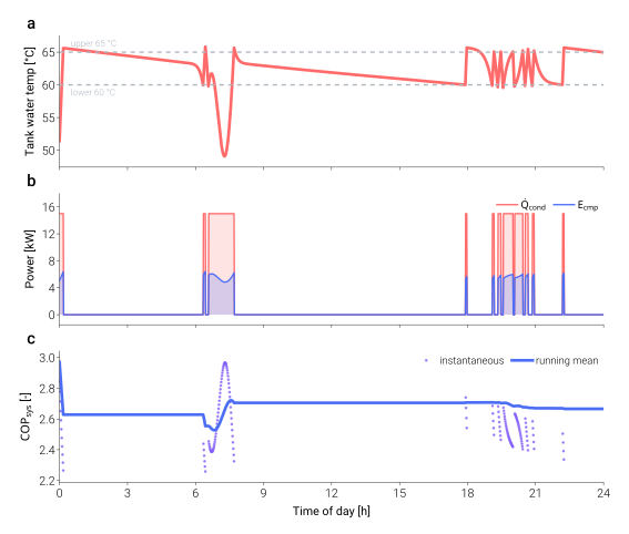
24-hour run of the ASHPB reference case with two DHW draws (07:00 and 20:00) and a sinusoidal outdoor temperature. Generated by scripts/visualization/dynamic_24h_timeseries.py.

What the result contains

analyze_dynamic returns a pandas.DataFrame with one row per time step. The columns are the same units-bracketed keys you get from analyze_steady, grouped roughly into:

• Cycle state points — P_ref_* pressures, T_ref_* temperatures at compressor / expander / evaporator / condenser nodes.

• Energy flows — Q_ref_tank [W], Q_ref_ou [W], E_cmp [W], fan / pump auxiliary power.

• Tank state — T_tank_w [°C], level [-].

• Figures of merit — cop_ref [-], cop_sys [-].

You can pull any of these out by name once the run finishes:

# Daily-average system COP, skipping the first hour of warm-up
df_steady = df.iloc[60:]
print(f"Daily COP_sys: {df_steady['cop_sys [-]'].mean():.2f}")

For the full column list, df.columns.tolist() after a short run is the fastest reference.

Common next moves

• Pass real weather to T0_schedule (hourly data resampled to dt_s) and a realistic DHW profile to dhw_usage_schedule.

• Save the run to disk by passing result_save_csv_path="run.csv".

• For solar-coupled or PV/ESS variants, instantiate the corresponding subclass (ASHPB_STC_preheat, ASHPB_STC_tank, ASHPB_PV_ESS, or the GSHPB counterparts) and pass the additional schedules (I_DN_schedule, I_dH_schedule, T_sup_w_schedule) as documented under Air-source heat pump boiler (ASHPB) and Ground-source heat pump boiler (GSHPB).

Note

analyze_dynamic uses a fully implicit time-stepping scheme — fsolve solves for [T_next, level_next] at every step. This makes the integrator robust to large dt_s values, but a 1-minute step is a safe default for first runs.

Last updated Jul 01, 2026